Category Archives: Lab blog

GPU

Creating a conda environment for GPU programming with pytorch and tensorflow

After a few mis-steps, here is how I set up a conda environment to use in Jupyter with tensorflow, pytorch, and using the GPU.

As a note, I do this on the node with the GPU, so that things (hopefully) compile correctly!

1. Create an environment

First, create a new environment for tensorflow and friends, and activate it.

mamba create -n gpu_notebook cudatoolkit tensorflow nvidia::cuda pytorch torchvision torchaudio pytorch-cuda -c pytorch -c nvidia
mamba activate gpu_notebook

2. Install the python libraries

Install the usual suspect python packages that you will probably want to use. For convenience, I usually put these in a file in my
Git repo called requirements.txt.

$ cat requirements.txt 
jupyter
matplotlib
natsort
numpy
pandas
scipy
scikit-learn
seaborn
statsmodels
pip install -r requirements.txt

3. Reame your jupyter kernel

When you open jupyter there is a list of kernels that you can connect to. (If you have a window open that list will be on the top right.) If you rename your jupyter kernel it makes it
much easier to find the kernel associated with this conda environment. The default name is something like Python 3 which is not helpful if you have lots of them!

a. Find where your kernel is installed

This command shows your jupyter kernels

jupyter kernelspec list

You’ll see your kernel(s) and the locations of them. In the location listed there is a file called kernel.json.

b. Edit that file:

vi $HOME/miniconda3/envs/gpu_notebook/share/jupyter/kernels/python3/kernel.json

c. Change the name to be meaningful

Change the value associated with the display_name key. Set it to something meaningful so you can find it in your browser!

4. Set up the XLA_FLAGS environment variable.

This was essential for me to get tensorflow working. There is a directory somewhere in your conda environment with the libdevice library that is needed. For my installation that was in nvvm/libdevice/libdevice.10.bc. Of course you can find yours with:

find ~/miniconda3/ -name libdevice

You want to set the XLA_FLAGS variable to point to the base of the nvvm folder. This command sets it inside the conda environment so it is always set when the conda environment is activated, and unset when it is deactivated.

conda env config vars set XLA_FLAGS=--xla_gpu_cuda_data_dir=$HOME/miniconda3/envs/gpu_notebook

5. Activate the environment

Don’t forget to submit this to a node with GPU capabilities!

statsmodels.mixedlm Singular Matrix error

When building linear mixed models with Python’s statsmodules module, I repeatedly, and often incoherently, ran into np.linalg.LinAlgError errors that are Singular matrix errors.

There are a couple of things to check for with these errors:

First, drop any rows where there are NaN values for the predictors:

e.g. if your predictors are in a list called predictors, try this

df= df.dropna(subset=predictors)

Second, remove any columns whose sum is zero:

to_drop = list(df.loc[:,df.sum(axis=0) <1].columns)
df.drop(columns=to_drop)

Third, now that you have dropped columns, make sure they are still in your predictors. Something like

updated_predictors = list(set(predictors).intersection(set(df.columns)))

Finally, when all that doesn’t work, you should try different methods to fit the model. These are the methods I currently use, and I try them in this order and save the results for the first one that completes.

results = None
for meth in 'bfgs', 'lbfgs', 'cg', 'powell', 'nm':
    try:
        result = model.fit(method=meth)
        print(f"Method {meth} PASSED", file=sys.stderr)
        break
    except np.linalg.LinAlgError as e:
        print(f"Method {meth} failed", file=sys.stderr)
if results:
    print(results.summary)
node.js logo

Installing node.js and nvm on WSL

I needed an updated node.js on my WSL … for some reason ubuntu 20 has quite an old version.

First, as sudo, I removed all the old versions to avoid any conflicts:

apt purge nodejs
apt auto-remove

The purge command completely removes it, while the autoremove removes any dependencies. That should be optional, because those should work once we install the new node.js versions, but YMMV.

Next, install the node.js installer, called nvm for node version manager

To begin, set up your install location. For a single install it should be in ~/.nvm but for a site-wide install, you might want to install nvm in /usr/local/nvm.

Put these lines in your ~/.bashrc

export NVM_ROOT_DIR=$HOME/.nvm
# export NVM_ROOT_DIR=/usr/local/nvm ## << use this version if you are doing a site wide install
export NVM_DIR=$HOME/.nvm
[ -s "$NVM_ROOT_DIR/nvm.sh" ] && . "$NVM_ROOT_DIR/nvm.sh"
[ -s "$NVM_ROOT_DIR/bash_completion" ] && . "$NVM_ROOT_DIR/bash_completion"
NVM_BIN=$HOME/.nvm/versions/node/v23.3.0/bin ## << you may need to change this line
NVM_INC=$HOME/.nvm/versions/node/v23.3.0/include/node ## << you may need to change this line
export PATH=$NVM_DIR:$NVM_BIN:$PATH

Download nvm and get the files you want:

git clone https://github.com/nvm-sh/nvm.git
mkdir -p $NVM_ROOT_DIR
cp nvm/nvm.sh nvm/bash_completion $NVM_ROOT_DIR

Now, reload your bash settings

source ~/.bashrc

You should be able to run the nvm commands:

which nvm
nvm ls

To install node.js use nvm install

nvm install node

If you see this error:

wsl -bash:  node: cannot execute binary file: Exec format error

then try installing a different version

node install --lts 

For me, using the default node install node didn’t work because of the binary file Exec format error, while using node install --lts worked like a charm!

Migrating from snakemake 7 to snakemake 8

I finally bit the bullet and migrated from snakemake 7 to snakemake 8. The short answer its not too hard!

First, install the executor plugin for snakemake using mamba:

mamba install snakemake-executor-plugin-cluster-generic

Next, edit your config file and change the following:

If you have a cluster: section, change that to cluster-generic-submit-cmd:

Add the line:

executor: cluster-generic

You need to remove these lines if you have them:

cluster-status
use-conda
conda-frontend

Here is my current snakemake config file

# non-slurm settings

conda-prefix: ~/.config/snakemake/conda/

# slurm settings

jobs: 600

executor: cluster-generic
cluster-generic-submit-cmd:
  mkdir -p logs_slurm/{rule} &&
  sbatch
    --cpus-per-task={threads}
    --mem={resources.mem_mb}
    --output=logs_slurm/{rule}/{jobid}.out
    --error=logs_slurm/{rule}/{jobid}.err
    --job-name=smk-{rule}
    --time={resources.runtime}
    --parsable

default-resources:
  - mem_mb=2000
  - runtime=7200
  - load_superfocus=0
  - load_kraken=0
  - load_onehundred=0

resources: [load_superfocus=100, load_kraken=100, load_onehundred=100]
local-cores: 32
latency-wait: 60
shadow-prefix: /scratch/user/edwa0468
keep-going: False
max-jobs-per-second: 20
max-status-checks-per-second: 10
scheduler: greedy

restart-times: 1

Global Phage Host Prediction Consortium

White Paper

Robert Edwards, Flinders University

September 2023

For comment

Please contact Rob Edwards (robert.edwards@flinders.edu.au)

Executive Summary

Infectious diseases are already one of the leading causes of mortality, and the rapid spread of antibiotic resistant bacteria is worsening this threat. Phage therapy is the most promising treatment to tackle the global threat of antimicrobial-resistant bacteria. However, numerous hurdles prevent its widespread implementation. The major benefit of phages is that they are highly specific, infecting only one or a few kinds of bacteria. However, this specificity defines one of the major hurdles: identifying, and accessing, the phages that might treat a patient. Currently, we have to ship the patient’s bacteria around the world to identify phages that might treat it, and then ship candidate phages back to where the treatment is needed. However, we are on the cusp of being able to choose appropriate therapeutic phages based on genome sequencing alone. This will open a new area for phage therapy: phages on demand. As Jean-Paul Pirnay describes it, PhageBeam to send phages via the internet. We should be able to sequence a patient’s bacterial isolate and use machine learning to identify the phage sequences that are most likely to infect that bacterium. Immediately, this would remove one step: the candidate phages could be retrieved and tested. In the long term, those phages could be synthesised locally and tested on the patient’s infection much faster than is currently possible. This project will enable scientists in less developed countries, will discover fundamentals of phage biology, and will save lives by reducing the threat of AMR.

Current State of the Art

Phages are being used worldwide to treat antimicrobial-resistant bacterial infections. However, successfully using a phage to kill bacteria depends on numerous factors: recognition of capsular polysaccharides (CPS) and lipopolysaccharides (LPS) on the cell surface; recognition of the bacterial receptor by the phage receptor binding protein; DNA translocation from the phage into the cell, and evasion of CRISPR/Cas and restriction/modification systems; eluding the bacterial defence mechanisms; replication; packing; and cell lysis. In the millions of years of evolution between bacteria and phages, they have both developed an arsenal to stop the other, and weapons to stop that arsenal. We know many of the actors that drive this warfare: there are approximately 200 bacterial defence mechanisms described so far, and almost as many anti-defence mechanisms. All of this makes it impossible, a priori, to predict which phage will infect which bacteria, based on the genome sequences alone.

What the field needs

That prediction is not impossible! Given enough sequenced phages and enough sequenced bacteria, we can build machine learning algorithms to predict which phages successfully kill which bacteria, and importantly, those algorithms will teach us why phages can, or cannot, kill a bacterium. From this, we can learn new bacterial defence mechanisms (e.g., CRISPR/Cas), new phage attack mechanisms, the role of prophages in regulating these interactions, the nature of the bacterial-CPS and bacterial-LPS interactions, and more about fundamental phage biology. We can use this information to select a suitable phage to treat a patient’s bacterial infection, identify where that phage is in the world, and speed up finding phages to cure infections.

The unknowns, which we can’t answer right now, are how may phages is enough, and how many bacteria is enough? We can’t answer these questions because we don’t have the underlying datasets needed to tackle this important challenge. This project will deliver those datasets.

How can we deliver enough data to create accurate machine learning algorithms?

We need to generate a massive dataset that covers the genomes of phages, the genomes of the bacteria, and the efficiency of plating of each phage on each bacterium (i.e., how many plaques does it form?). Although this sounds like an insurmountable challenge, the hardest part of this has already been done by labs all over the world: they have identified thousands of phages and compared them to thousands of bacteria because this is a cheap and easy experiment that only requires a few laboratory supplies. Almost every phage lab in the world does this experiment: They isolate a new phage from the environment, test it against all the bacteria in their collections and generate a matrix where the rows are bacterial species, the columns are phage species, and the cell contents are a number representing the efficiency of plating. If we can sequence the bacteria and phages that constitute those tables, and capture the sequence data, EOP data, and other data that is generated we can build machine learning algorithms that will predict phage infectivity.

We propose to distribute Oxford Nanopore Mk1C DNA sequencers to phage labs all over the world and have them sequence the bacteria and the phages that they are isolating. We will ask that they provide that data to our central database, and we will encourage them to publish their sequences and analyses of their results and make their data publicly available (e.g., through the NCBI, ENA, and DDBJ). We specifically propose the Mk1C because it will enable researchers in less developed countries to become engaged in this research experience. The Mk1C is a standalone unit that does not require internet access which has been a limiting factor in many countries (e.g., India, Africa) to using the Mk1B MinION

We estimate that one Nanopore Mk1C sequencing run can be used to sequence between 15 and 46 bacterial genomes together with 50 phage genomes.

We will build the computational infrastructure to allow the collaborators to upload their phage and bacterial genomes, the efficiency of plating metrics, and other data they measure (e.g., one-step growth curves, synograms, etc.) and to integrate them into a publicly available resource. All sequences will be annotated and shared using the RAST database at Argonne National Labs/ the University of Chicago, to ensure consistent and accurate annotations. RAST is the most widely used phage and bacterial genome annotation resource. We will complement those analyses with local analyses using new computational tools we will develop for this process.

Estimated Budget

For each sample, we estimate that the budget will be (prices are current in AUD):

  • $845 – 50 Bacterial DNA extraction
  • $1,289 – 50 Phage DNA extractions
  • $699 – V14 barcoding kit for 96 samples
  • $900 – for one V14 flow cell
  • $218 – 100 assays Qubit

Total: $3,951 (approximately US$2,500 // €2,400)
Therefore, with ~€100,000 we will provide approximately 40 sequencing kits globally, and sequence approximately 2,000 bacterial and phage genomes.

bash

Human Readable Numbers

There is an easy convenience to using human readable numbers. Instead of a number like 1,099,511,627,776 you can use 1T. Instead of 1,073,741,824 you can use 1G and instead of 1,024 you can use 1K (that 1K = 1,024 is why the other numbers don’t end with multiple zeros).

But how do you do some (simple) math with human readable numbers, like adding up a list?

This is where numfmt comes to your aid.

For example, lets make a list of numbers:

259G
1.1G
692G
5.5G
5.3G
140M
30G
302G
222G
281M
1.9G
60G
2.2T

If we put those in a file called sizes.txt we can sum them with a simple command like this:

cat sizes.txt | numfmt --from=iec | awk 's+=$1 {} END {print s}'  | numfmt --to=iec

The --from=iec converts the numbers from human readable format to numbers, the awk adds the numbers, and then the second numfmt converts the sum back to a human readable number,

phyloseq logo

Converting phyloseq objects to read in other languages

Phyloseq is an R package for microbiome analysis that incorporates several data types.

Occassionally our colleagues share a phyloseq object with as an .rds file (R Data Serialization format). It is quite simple to convert that for use in other languages (e.g. python or even Excel!)

Converting the data to .tsv format

This approach requires an R installation somewhere, but we don’t need many commands, so you can probably use a remote R installation on a server!

If you have not yet installed phyloseq, you can do so with bioconductor:

if (!require("BiocManager", quietly = TRUE))
install.packages("BiocManager")
BiocManager::install("phyloseq")

Next, we load the phyloseq package and read the .RDS file:

library("phyloseq");
packageVersion("phyloseq"); # check the version we are using
# you may need to use setwd("C:/Users/username/Downloads") to move to whereever you downloaded the file!
p <- readRDS("phyloseq.rds"); # change the filename here! 
print(p)

This will print typical output from a phyloseq object like:

phyloseq-class experiment-level object
otu_table()   OTU Table:         [ 3210 taxa and 11 samples ]
sample_data() Sample Data:       [ 11 samples by 12 sample variables ]
tax_table()   Taxonomy Table:    [ 3210 taxa by 7 taxonomic ranks ]

These are our base phyloseq objects, and we can explore them:

print(otu_table(p))
print(sample_data(p))

And we can also write them to tab separated text in a .tsv file:

write.table(otu_table(p), "p_otu.tsv", sep="\t")
write.table(sample_data(p), "p_sample.tsv", sep="\t")
write.table(tax_table(p), "p_tax.tsv", sep="\t")

Read those files into Python

You can now use pandas to read those files into Python:

import pandas as pd

otu = pd.read_csv("p_otu.tsv", sep="\t")
otu

# sometimes the sample metadata has characters that can't be read using `utf-8` so we have to use `latin-1`
samples = pd.read_csv("p_sample.tsv", sep="\t", encoding='latin-1')
samples

tax = pd.read_csv("p_tax.tsv", sep="\t")
tax
git logo

Git change remote from https to ssh

Here’s how to change your remote from https to ssh.

Start by checking your current remote:

git remote -v

and this will list your remotes for both push and fetch.

To set a remote, you can use

git remote set-url origin git@github.com:username/project.git

and then use remote again to confirm:

git remote -v

now your git pull and git push will work as you expect!

bash

Use column to display tsv files in columns

If you have a tab separated file and view it in a pager like less or more, the columns never line up. Here is a simple way to make those columns appear correct.

column -t file.tsv

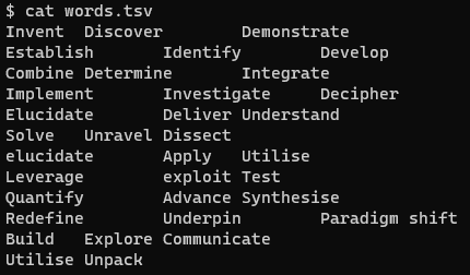
For example, here is a file with three columns of words, displayed with cat

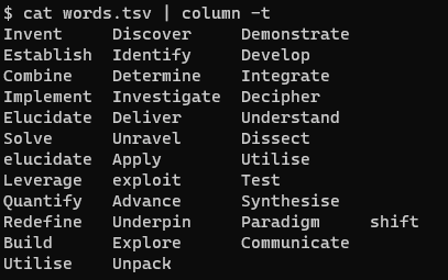
If we pass that to column with the -t option to detect the columns, we get nicely organised columns:

However, note that this is not exactly correct, notice that “Paradigm shift” has been split into two columns because the -t option uses whitespace by default, so to display the columns using tabs, we need to add a -s option:

column -t -s$'\t'

bash

awk use tab as input separator

By default, awk uses any whitespace to separate the input text. You can use the same construct as perl to change the input Field separator:

cat file.tsv | awk -F"\t" '!s[$1]'

The above example will split a file on tabs and then print the unique entries in the first column.